Understanding regularization
Contents
2. Understanding regularization
2.1. Karush-Kuhn-Tucker Optimization
Using regularization in the training of a model is adding a constraint to the loss function. To do that we need to generalize the method of Laplace multipliers, namely the Karush-Kuhn-Tucker conditions (KKT conditions).
Let \(l(x)\) be loss function, the function we desire to minimize. The solution space, \(\mathbb{S}\) is restricted in two ways:
where:
The \(g^{(i)}(x)\) equations are called equality constraints;
and \(h^{(j)}(x)\) inequality constraints.
The generalized Lagrangian is
where \(\lambda_{i}\) and \(\alpha_{j}\) are the KKT multipliers.
So our objective is to minimize \(L(\mathbf{x},\mathbf{\lambda},\mathbf{\alpha})\) with respect to \(\mathbf{x}\) and maximize it w.r.t. \(\mathbf{\lambda}\) and \(\mathbf{\alpha}\):
Let us see an example with an inequality constraint:
We want to minimize \(l(x) = x^{2}+x+1\) subjected to \(h(x) = x \ge 0\). Then the Generalized Lagrangian is
The minus sign is added to transform the inequality sign (from \(\ge\) to \(\le\)). We have \(\alpha \ge 0\), \(h(x) \ge 0\) and \(\alpha h(x) = 0\).
If \(\alpha = 0 \), its minimum allowed value, \(x = 1/2\). To respect the constraint tha maximum value of \(\alpha\) is \(1\). Then we have \(0 \le \alpha \le 1\), but \(\alpha = 1\) allows \(x\) to be zero. Let us compare \(l\) and \(L\) with their minimum values.
import numpy as np
import matplotlib.pyplot as plt
np.random.seed(42)

x = np.linspace(-2,2,50)
l = lambda x: x**2 + x + 1
h = lambda x: x
L = lambda x,a: l(x) - a*h(x)
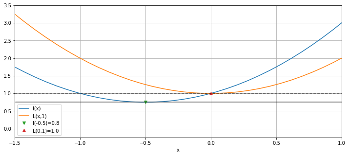
We see the constraint raises the minimum value of \(l(x)\). This is the same behavior we expect from a regularization to prevent overfitting. The example above seems silly since there is only one minimum. Let us see another example.
2.2. Example - Regularizing a neural network
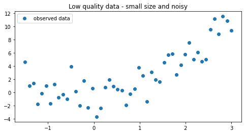
x = np.linspace(-1.5,3,50)
noise = np.random.normal(0,2.0,size=len(x))
y = 0.2 + 0.5*x + x**2 + noise
2.2.1. Define neural net architecture and training method
import torch
import torch.utils.data as Data
import torch.nn as nn
import torch.optim as optim

torch.manual_seed(0)
ngpu = 1
device = torch.device("cpu")

class Net(nn.Module):
    def __init__(self,h_dim=1,ngpu=ngpu):
        super(Net, self).__init__()
        self.h_dim = h_dim
        self.hidden = nn.Linear(1, self.h_dim)
        self.act1 = nn.ReLU()
        self.out = nn.Linear(self.h_dim, 1)

    def forward(self, x):
        h = self.act1(self.hidden(x))
        return self.out(h)

def init_weights(m):
    if type(m) == nn.Linear:
        torch.nn.init.xavier_normal_(m.weight).to(device)
        m.bias.data.fill_(0.001)

def define_model(model_class,h_dim):
    net = model_class(h_dim).to(device)
    if (device.type == 'cuda') and (ngpu > 1):
        net = nn.DataParallel(net, list(range(ngpu)))

    net.apply(init_weights)
    learning_rate = 0.001
    net_optimizer = optim.Adam(net.parameters(),lr=learning_rate)
    return net,net_optimizer

def create_loader(X,y,batch_size=5,workers=12):
    torch_dataset = Data.TensorDataset(X,y)
    loader = Data.DataLoader(
            dataset = torch_dataset,
            batch_size = batch_size,
            shuffle=True)
    return loader

def train_model(model,optimizer,epochs=200,regularize=False,a=0.01):
    mse_loss = nn.MSELoss()
    for epoch in range(epochs):
        loss_ = []
        for _, (X_train,y_train) in enumerate(loader):
            X_train = X_train.view(-1,1).to(device)
            y_train = y_train.view(-1,1).to(device)
            y_pred = model(X_train)
            # custom loss with regularization by norm of weights
            if regularize == True:
                l2_reg = None
                for W in model.parameters():
                    if l2_reg is None:
                        l2_reg = W.norm(2)
                    else:
                        l2_reg = l2_reg + W.norm(2)
                loss = mse_loss(y_pred,y_train) + a*l2_reg
            else:
                loss = mse_loss(y_pred,y_train)
            loss.backward()
            optimizer.step()
            optimizer.zero_grad()
    return model
2.2.2. Dataloader
x_t = torch.Tensor(x.reshape(-1,1)).type(torch.FloatTensor)
y_t = torch.Tensor(y).type(torch.FloatTensor)

loader = create_loader(x_t,y_t,batch_size=50,workers=12)
2.2.3. Train models
h_dim = 10000
epochs = 500
models = [define_model(Net,h_dim_) for h_dim_ in [h_dim]*5]
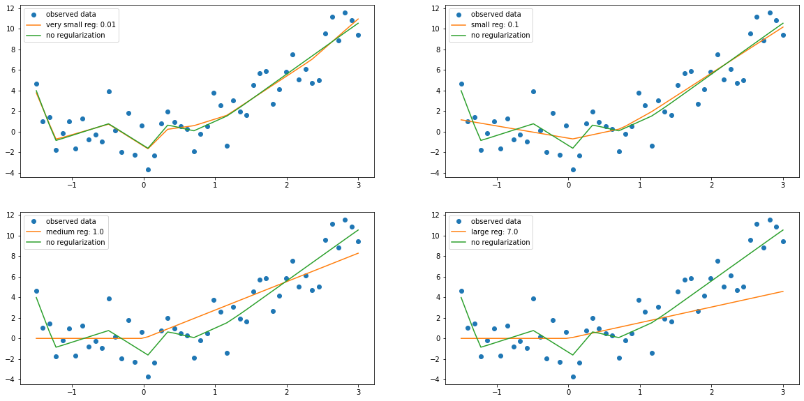
regularization_factors = [0.01,0.1,1.0,7.0]
model_reg_1 = train_model(models[0][0],models[0][1],epochs,True,regularization_factors[0])
model_reg_2 = train_model(models[1][0],models[1][1],epochs,True,regularization_factors[1])
model_reg_3 = train_model(models[2][0],models[2][1],epochs,True,regularization_factors[2])
model_reg_4 = train_model(models[3][0],models[3][1],epochs,True,regularization_factors[3])
model_non_reg = train_model(models[4][0],models[4][1],epochs,False)
2.2.4. Evaluation
y_pred = []
y_pred.append(model_reg_1(x_t.view(-1,1).to(device)).detach())
y_pred.append(model_reg_2(x_t.view(-1,1).to(device)).detach())
y_pred.append(model_reg_3(x_t.view(-1,1).to(device)).detach())
y_pred.append(model_reg_4(x_t.view(-1,1).to(device)).detach())
y_pred.append(model_non_reg(x_t.view(-1,1).to(device)).detach())

plt.figure(figsize=(20,10))
plt.subplot(221)
plt.plot(x_t.cpu().numpy(),y_t.cpu().numpy(),'o',label="observed data")
plt.plot(x_t.cpu().numpy(),y_pred[0].detach().cpu().numpy(),label=f"very small reg: {regularization_factors[0]}")
plt.plot(x_t.cpu().numpy(),y_pred[4].detach().cpu().numpy(),label="no regularization")
plt.legend(loc=0)
plt.subplot(222)
plt.plot(x_t.cpu().numpy(),y_t.cpu().numpy(),'o',label="observed data")
plt.plot(x_t.cpu().numpy(),y_pred[1].detach().cpu().numpy(),label=f"small reg: {regularization_factors[1]}")
plt.plot(x_t.cpu().numpy(),y_pred[4].detach().cpu().numpy(),label="no regularization")
plt.legend(loc=0)
plt.subplot(223)
plt.plot(x_t.cpu().numpy(),y_t.cpu().numpy(),'o',label="observed data")
plt.plot(x_t.cpu().numpy(),y_pred[2].detach().cpu().numpy(),label=f"medium reg: {regularization_factors[2]}")
plt.plot(x_t.cpu().numpy(),y_pred[4].detach().cpu().numpy(),label="no regularization")
plt.legend(loc=0)
plt.subplot(224)
plt.plot(x_t.cpu().numpy(),y_t.cpu().numpy(),'o',label="observed data")
plt.plot(x_t.cpu().numpy(),y_pred[3].detach().cpu().numpy(),label=f"large reg: {regularization_factors[3]}")
plt.plot(x_t.cpu().numpy(),y_pred[4].detach().cpu().numpy(),label="no regularization")
plt.legend(loc=0)
plt.show()