Ranknet - Teacher-Student strategy
Contents
3. Ranknet - Teacher-Student strategy
Let \(\mathcal{D} = \{(\mathbf{x}_{i},y_{i}) | i \in \{1,2,...,N\}, \mathbf{x}_{i} \in \mathbf{X} \subset \mathbb{R}^{m} \text{ and } y_{i} \in \mathbb{R}^{1} \}\) be a dataset with \(m\) features, 1 label and \(N\) obervations.
Let us split \(\mathcal{D}\) in terms of features: \(\mathbf{x}_{i,s} \in \mathbf{X}_{s}\) is n-dimensional and \(\mathbf{x}_{i,t} \in \mathbf{X}_{t}\) is m-dimensional, where \(n<m\) such that \(\mathbf{X}_{s} \subset \mathbf{X}_{t}\). Actually \(\mathbf{X}_{t}\) may be \(\mathcal{D}\) itself. Thus \(\mathbf{X}_{s}\), which we will call Student set, is a partition of the dataset, i.e., a matrix containing all the observations but not all the features available in \(\mathbf{X}_{t}\), called Teacher set.
Since \(\mathbf{X}_{t}\) is larger it has more information than \(\mathbf{X}_{s}\). We face the following problem:
Proposition 3.1
We could train a model with \(\mathbf{X}_{t}\), but it is too complex and expensive to put it on production. Maybe the prediction time must be very small and using the set of all features is an impeditive. Thus, if we could train a less complex model with less features the prediction time would be smaller.
We could also achieve that using a dimensionality reduction model, but there is another options like the one we will see here, the Teacher-Student method of training.
Note
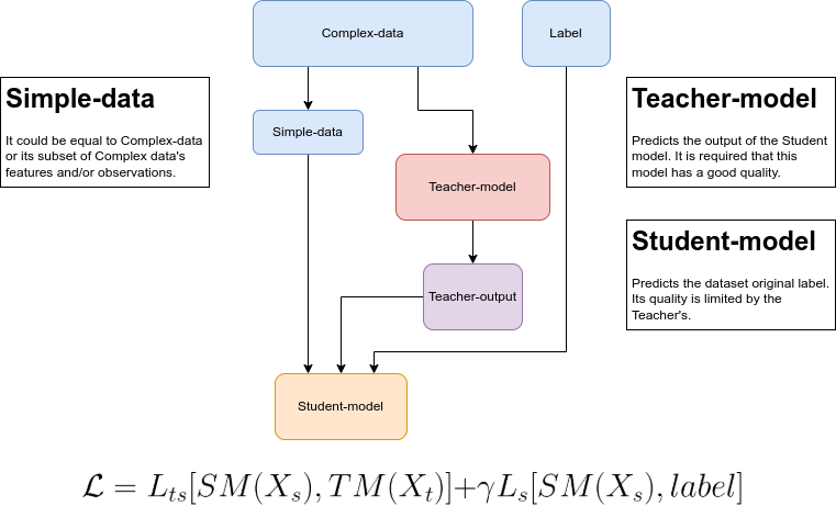
This is just one method for training a model and can be used in practically all applications, not only in ranking problems. There are two main approaches as we can see in the following diagrams:
Note
Method 1:
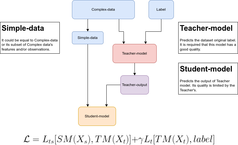
Note
Method 2:
Assuming we are solving a ranking problem, the label represents some kind of relevance. In this example we will assume that a label can have two values, \(\{0,1\}\). So the definition above is changed to \(y_{i} \in \{0,1\}\), where \(1\) means more relevance than \(0\). In future examples we will see other kinds of relevance.
As mentioned before, we need two models: teacher model (TM) and student model (SM). In this formulation these models can be any gradient based regression models you like.
To train a Ranknet one needs in each iteration to sample a pair of observations, one more relevant than the other. We will refer to them as:
\(\mathbf{x}_{i,s,r}\): features vector of observation \(i\) from the Student set which has relevance \(r\);
\(\mathbf{x}_{i,t,r}\): features vector of observation \(i\) from the Teacher set which has relevance \(r\).
In each sampling iteration we always need \(\left( \mathbf{x}_{i,s,1},\mathbf{x}_{j,s,0} \right)\) for the SM and \(\left( \mathbf{x}_{i,t,1},\mathbf{x}_{j,t,0} \right)\) for the TM. Notice that we are using only two observations here, \(i\) and \(j\). The models output for these vectors are the scores, denoted as:
\(s_{i,s}\): the score assigned to observation \(i\) by the Student model;
\(s_{i,j}\): the score assigned to observation \(i\) by the Teacher model.
3.1. The Teacher-Student algorithm for the Ranknet
In order to use method 1 we need the following algorithm:
Algorithm 3.1 (Ranknet Teacher-Student)
Init TM and ST models.
Repeat for T epochs:
Sample \(\mathbf{x}_{i,s,1},\mathbf{x}_{j,s,0},\mathbf{x}_{i,t,1},\mathbf{x}_{j,t,0} \sim \mathcal{D}\)
Train and update TM:
Compute scores
\(s_{i,t} = TM(\mathbf{x}_{i,t,1})\)
\(s_{j,t} = TM(\mathbf{x}_{j,t,0})\)
Compute likelihood, \(\sigma(s_{i,t},s_{j,t})\)
\(prob = sigmoid(s_{i,t},s_{j,t})\)
Compute loss:
\(\mathcal{L}_{teacher} \left( prob,1 \right)\)
Update TM:
\(\theta_{t} \leftarrow \theta_{t} - \gamma_{t} \nabla \mathcal{L}_{teacher}\)
For try in num_tries (it can be 1):
Train and update SM to predict the same scores as TM:
Compute TM scores
\(s_{i,t} = TM(\mathbf{x}_{i,t,1})\)
\(s_{j,t} = TM(\mathbf{x}_{j,t,0})\)
Compute SM scores
\(s_{i,s} = SM(\mathbf{x}_{i,s,1})\)
\(s_{j,s} = SM(\mathbf{x}_{j,s,0})\)
Compute two losses:
\(\mathcal{L}_{student,i} \left( s_{i,s},s_{i,t} \right)\)
\(\mathcal{L}_{student,j} \left( s_{j,s},s_{j,t} \right)\)
\(\mathcal{L}_{student} = \mathcal{L}_{student,i} + \mathcal{L}_{student,j}\)
Update SM:
\(\theta_{s} \leftarrow \theta_{s} - \gamma_{s} \nabla \mathcal{L}_{student}\)
The prediction quality of the student will not be as good as the one from the teacher, but it could be a small price to pay for using a simpler model. If the SM score are not converging to similar value as those of TM the num_tries parameter can be adjusted to let the student “study” more. There is no mistery about the SM loss functions, we can use any like mean squared error.